本文讨论量子噪声。

参考文献：

1. A.~A. Clerk, M.~H. Devoret, S.~M. Girvin, F. Marquardt, and R.~J. Schoelkopf, Introduction to Quantum Noise, Measurement and Amplification, Rev. Mod. Phys. 82, 1155 (2010).
2. Nielsen, Michael A., and Isaac L. Chuang. Quantum Computation and Quantum Information: 10th Anniversary Edition. Cambridge: Cambridge University Press, 2010.
3. J. R. Johansson, P.D. Nation, and F. Nori, “QuTiP 2: A Python framework for the dynamics of open quantum systems”, Comp. Phys. Comm. 184, 1234 (2013).

1. 经典噪声和量子噪声

1.1 经典噪声

  一个电压信号 \(V(t)\) ，\(\langle V(t)\rangle=0\)，服从正态分布。

自相关函数（autocorrelation function)

$$ G_{VV}(t-t’)=\langle V(t)V(t’) \rangle $$

   自相关函数随时间衰减，特征时间为\(\tau_c\)。

功率谱密度函数（spectral density)

$$ S_{VV}[\omega]=\int_{-\infty}^{+\infty}\mathrm{d}t e^{i\omega t}G_{VV}(t) \tag{1.1} $$

  从功率谱密度求自相关函数，做一个逆傅立叶变换：

$$ G_{VV}(t)=\int_{-\infty}^{+\infty}\frac{\mathrm{d}\omega}{2\pi} e^{-i\omega t}S_{VV}[\omega] $$

  自相关时间极短，即白噪声（white noise），功率谱密度为常数： $$ S_{VV}[\omega]=\sigma^2 $$ $$ G_{VV}(t)=\sigma^2 \delta(t) $$

  经典噪声的功率谱密度为偶函数。 $$ S_{VV}[\omega]=S_{VV}[-\omega] $$

1.2 经典噪声测量

1 MHz 以下 直接测量

1 GHz 以上

1.3 量子噪声

功率谱密度函数（spectral density)

$$ S_{xx}[\omega]=\int_{-\infty}^{+\infty}\mathrm{d}t e^{i\omega t}\langle \hat{x}(t)\hat{x}(0)\rangle \tag{1.2} $$

  量子噪声的功率谱密度不为偶函数。

$$ S_{VV}[\omega]\neq S_{VV}[-\omega] $$

其正频率部分与被谐振子吸收的受迫辐射能量相关，其负频率部分与谐振子发出的辐射能量相关。

2. 几个例子

  封闭孤立系统中的态变换可以用 Schrödinger 方程描述。

  对于开放系统，态的变换不是幺正变换，需要用主方程（master equation）描述。

Lindblad Master Equation

$$ \frac{\mathrm{d}\hat{\rho}}{\mathrm{d}t}=-\frac{i}{\hbar}[\hat{H},\hat{\rho}]+\sum_j \hat{L}_j\hat{\rho}\hat{L}_j^\dagger-\frac{1}{2}\{\hat{L}_j^\dagger\hat{L}_j, \hat{\rho}\} $$

2.1 激发态原子的自发辐射 Relaxation

  以二能级系统为例

$$ \hat{H}=\frac{\hbar\omega_q}{2}\hat{\sigma}_z $$

定义： $$\ket{\uparrow}\equiv\ket{1} $$

$$\ket{\downarrow}\equiv\ket{0} $$

Lindblad 算符 $$ \hat{L}=\sqrt{\gamma_r}\hat{\sigma}_-=\sqrt{\gamma_r}\ket{0}\bra{1} $$

假设初态为\(\ket{\psi}=\ket{1}\)，代入 Lindblad 方程计算。

省略计算过程得到：

$$ \hat{\rho}(t)=\begin{bmatrix} 1-e^{-\gamma_r t}&0\\ 0&e^{-\gamma_r t} \end{bmatrix} $$

用QuTiP模拟：

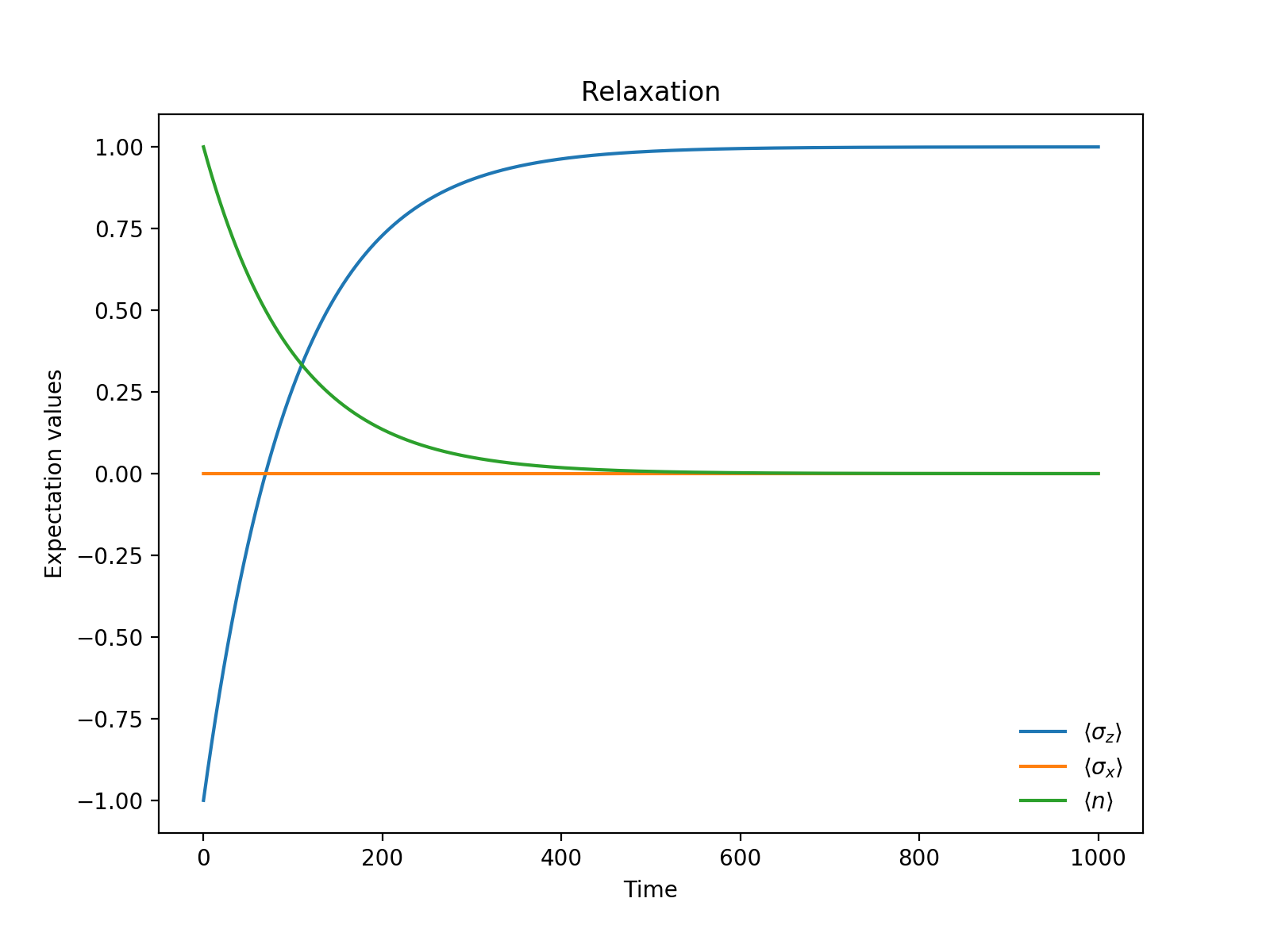
  最终趋向稳态\(\ket{0}\)。

代码如下：

 1
 2
 3
 4
 5
 6
 7
 8
 9
10
11
12
13
14
15
16
17
18
19
20
21
22
23
24
25
26
27
28
29
30
31
32
33
34
35
36

#!/usr/bin/env python3
# -*- coding: utf-8 -*-
"""
Created on Sun Aug 14 18:53:59 2022

@author: klucas
"""

from qutip import *
import numpy as np
import scipy.constants as C
import matplotlib.pyplot as plt

omega_q = 1e9
H = C.hbar / 2 * 1e12 * sigmaz()
psi0 = basis(2, 1)
gamma_r = 0.01
times = np.linspace(0.0, 1000.0, 10000)
result = mesolve(H, psi0, times, 
                 [np.sqrt(gamma_r) * Qobj([[0,1],[0,0]])], 
                 [sigmaz(), sigmax(), num(2)])

fig, ax = plt.subplots(figsize=(8,6), dpi=200)
ax.plot(times, result.expect[0])
ax.plot(times, result.expect[1])
ax.plot(times, result.expect[2])
ax.set_xlabel('Time')
ax.set_ylabel('Expectation values')
plt.title("Relaxation")
ax.legend((r"$\langle\sigma_z\rangle$", 
           r"$\langle\sigma_x\rangle$", 
           r"$\langle n \rangle$"), frameon = False)
plt.show(fig)

# 导出图片
fig.savefig("Relaxation.png")

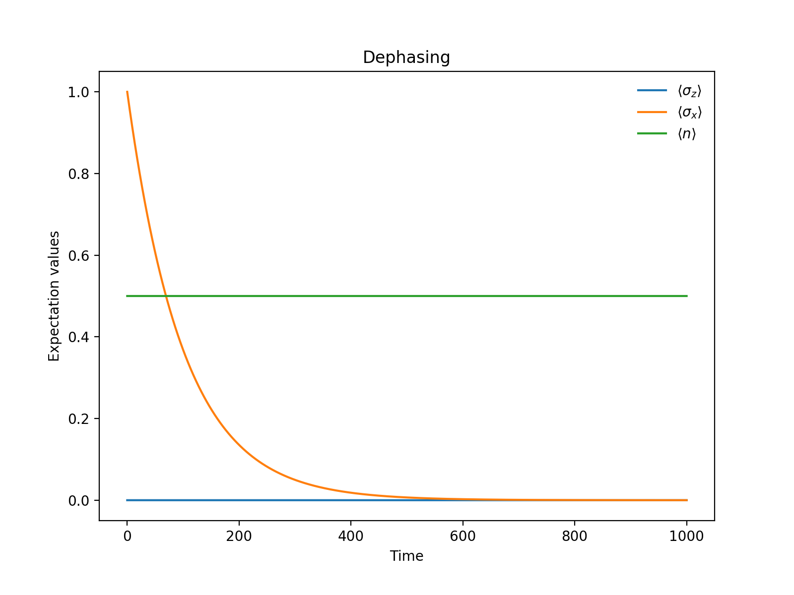
2.2 退相干 Dephasing

  描述退相干过程的 Lindblad 算符为：

$$ \hat{L}=\sqrt{\frac{\gamma_\phi}{2}}\hat{\sigma}_z=\sqrt{\frac{\gamma_\phi}{2}}(\ket{1}\bra{1}-\ket{0}\bra{0}) $$

假设初态为\(\ket{\psi}=\frac{1}{\sqrt2}(\ket{1}+\ket{0})\)，代入 Lindblad 方程计算。

省略计算过程得到：

$$ \hat{\rho}(t)=\begin{bmatrix} 1-\frac{1}{2}e^{-\gamma_r t}&\frac{1}{2}e^{-(\frac{\gamma_\phi}{2}+\gamma_r) t}e^{i\omega_q t}\\ \frac{1}{2}e^{-(\frac{\gamma_\phi}{2}+\gamma_r) t}e^{-i\omega_q t}&\frac{1}{2}e^{-\gamma_r t} \end{bmatrix} $$

用QuTiP模拟：

代码如下：

 1
 2
 3
 4
 5
 6
 7
 8
 9
10
11
12
13
14
15
16
17
18
19
20
21
22
23
24
25
26
27
28
29
30
31
32
33
34
35
36
37

#!/usr/bin/env python3
# -*- coding: utf-8 -*-
"""
Created on Mon Aug 15 13:55:55 2022

@author: klucas
"""

from qutip import *
import numpy as np
import scipy.constants as C
import matplotlib.pyplot as plt

omega_q = 1e9
H = C.hbar / 2 * 1e12 * sigmaz()
psi0 = (basis(2, 1)+basis(2,0)).unit()
gamma_r = 0.01
gamma_phi = 0.01
times = np.linspace(0.0, 1000.0, 10000)
result = mesolve(H, psi0, times, 
                 [-np.sqrt(gamma_phi / 2)  * sigmaz()], 
                 [sigmaz(), sigmax(), num(2)])

fig, ax = plt.subplots(figsize=(8,6), dpi=200)
ax.plot(times, result.expect[0])
ax.plot(times, result.expect[1])
ax.plot(times, result.expect[2])
ax.set_xlabel('Time')
ax.set_ylabel('Expectation values')
plt.title("Dephasing")
ax.legend((r"$\langle\sigma_z\rangle$", 
           r"$\langle\sigma_x\rangle$", 
           r"$\langle n \rangle$"), frameon = False)
plt.show(fig)

# 导出图片
fig.savefig("Dephasing.png")